How To Set Up A Pivot Table / Pivot Tables Better Excel Exporter For Jira Midori : To do so, highlight your entire data set (including the column headers), click insert on the ribbon, and then click the pivot table button.. Click the insert tab at the top of the excel window. Once you've entered data into your excel worksheet, and sorted it to your liking, highlight the cells you'd like to summarize in a pivot table. I changed the pivot table's name to sales. In the grouping dialog, please do the following options: Next, select the insert tab from the toolbar at the top of the screen.
I added the text shown in cell a1 in the figure below. To create a blank pivot table: The first step is to select a cell in the values area of the pivot table. In this example, we've selected cell a1 on sheet2. How to group pivot table dates.
Pivot Table Tips Exceljet from exceljet.net Now the pivot table is ready. Start the pivot table wizard. To create a blank pivot table: Click the relevant field item within the values area of the pivot table fields task pane. A create pivottable window should appear. Click the pivottable button on the left side of the insert ribbon. How to group pivot table dates. Click any single cell inside the data set.
After that, we will assign date and products to the rows label as well as the sales to the values section;
For the pivot table, data should be in the right and correct form. In this example, click on sum of salary item. While clicked inside a cell of the pivot table, visit the pivot table analyze tab of the ribbon, select the button for fields, items, and sets, and then click on calculated field. 2. Select a cell in the pivot table. Start the pivot table wizard. This action will prompt another window, which will show you some options about where you would like to place your pivot table. The first step to creating a pivot table is setting up your data in the correct table structure or format. Make sure your data is in columns with headers. From the insert tab, choose to insert a pivot table. select the pivot table fields such as salesperson to the rows and q1, q2, q3, q4 sales to the values. Next, select the insert tab from the toolbar at the top of the screen. To create a blank pivot table: This will greatly reduce the size of your pivot table. Once you've played around with the pivot table feature and gained some understanding of how the various options affect your data, then you can start creating a pivot table from scratch.
In the tables group, click on the tables button and select pivottable from the popup menu. Highlight your cells to create your pivot table. Setting up conditional formatting for pivot tables is a little different than it is for regular cells/ranges. This is the source data you will use when creating a pivot table. While clicked inside a cell of the pivot table, visit the pivot table analyze tab of the ribbon, select the button for fields, items, and sets, and then click on calculated field. 2.
Vba To Create A Pivot Table In Excel Ready To Use Macro Code from mk0excelchampsdrbkeu.kinstacdn.com This will greatly reduce the size of your pivot table. While creating a pivot table, make sure there will be no blank column or row. Another way to clone a pivot table is to copy the pivot table, and paste it somewhere else. After that, we will assign date and products to the rows label as well as the sales to the values section; Click the relevant field item within the values area of the pivot table fields task pane. The following is a list of components of a data table. Select any of the cells from your pivot table. First, i inserted several rows above the pivot table.
For the pivot table, data should be in the right and correct form.
Another way to clone a pivot table is to copy the pivot table, and paste it somewhere else. Choose where to place your pivot table after clicking that pivot table button, you'll be met with a popup that asks where you'd like to place your pivot table. Select the cells you want to create a pivottable from. Go to the ribbon and select the insert tab. The first way involved duplicating the worksheet that holds the pivot table. While creating a pivot table, make sure there will be no blank column or row. While clicked inside a cell of the pivot table, visit the pivot table analyze tab of the ribbon, select the button for fields, items, and sets, and then click on calculated field. 2. A create pivottable window should appear. Click the insert tab at the top of the excel window. If you are using excel 2003 or earlier, click the data menu and select pivottable and pivotchart report. Standard rules for pivot table data preparation start your data table in cell a1 (preferable) all columns must have header field names or titles (vital) header titles should be unique, although excel will add underscores suffixes to make them unique if you don't (preferable) After have created your pivot table, please right click any date in the pivot table, and select group from the context menu, see screenshot: I added the text shown in cell a1 in the figure below.
Click ok to close the dialog box. So in this post i explain how to apply conditional formatting for pivot tables. You can apply value filtering on pivot tables to show just the top performing customer (or product, city etc.). Click the insert tab at the top of the excel window. This will greatly reduce the size of your pivot table.
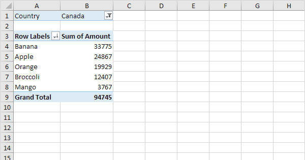
Pivot Tables In Excel Easy Excel Tutorial from www.excel-easy.com If you have a pivot table set up in worksheet with a title, etc., you can just right click the worksheet tab to copy the worksheet into the same workbook. Select any of the cells from your pivot table. The first way involved duplicating the worksheet that holds the pivot table. From the insert tab, choose to insert a pivot table. select the pivot table fields such as salesperson to the rows and q1, q2, q3, q4 sales to the values. Next, select the insert tab from the toolbar at the top of the screen. Select a cell in the values area. To create a blank pivot table: In the grouping dialog, please do the following options:
Select the cells you want to create a pivottable from.
To insert a pivot table, execute the following steps. Highlight the cell where you'd like to create the pivot table. Select the range of data for the pivot table and click on the ok button. Now the pivot table is ready. If you have a pivot table set up in worksheet with a title, etc., you can just right click the worksheet tab to copy the worksheet into the same workbook. This will greatly reduce the size of your pivot table. Go to insert tab → charts → pivot chart and select the chart which you want to use. Click any single cell inside the data set. Make sure your data is in columns with headers. Options > change source data; I changed the pivot table's name to sales. Your data shouldn't have any empty rows or columns. That pivottable's settings will be automatically imported and used in the future.